What the Future Holds

In the coming years, the population in the Intermountain West will likely continue to increase. Projected growth, in combination with a climate that is becoming increasingly variable, raises concerns about whether we will have enough water to meet everyone's needs.

Forecasting models help predict future supply and demand, as well as our vulnerability to disasters like floods and droughts. These models help communities prepare for the future. When communities better understand risks, they can make more informed water management decisions.

Forecasting water supply and demand is notoriously difficult. Water sources and needs change over time. They are influenced by multiple interrelated factors—like climate variability, population changes, water use policy, distribution technology, economic growth, environmental impact, agriculture demand, and water cost.

As technology and methods advance, forecasts are getting better. But because of the they involve so many dynamic variables, they will always have an element of uncertainty. Water managers can factor in this uncertainty by planning for a range of possible conditions.

To read more about how predictive models are used to create weather forecasts see What You Can Do With Models: Make Predictions
Water Supply Map

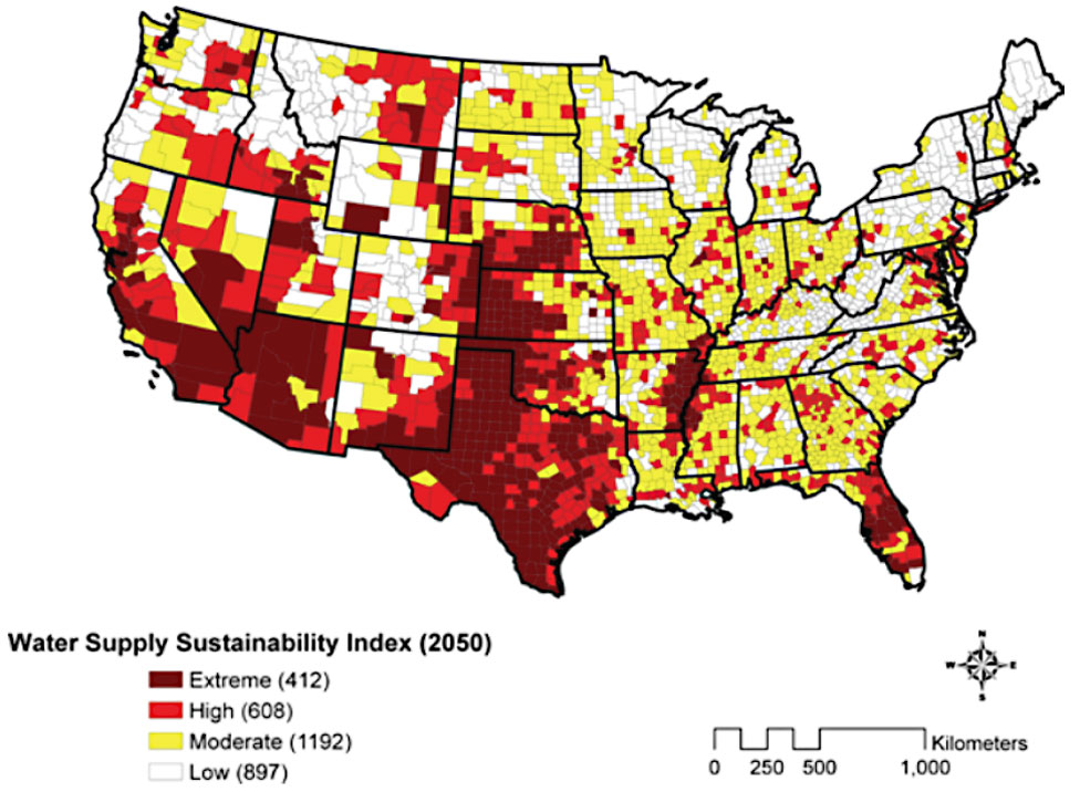
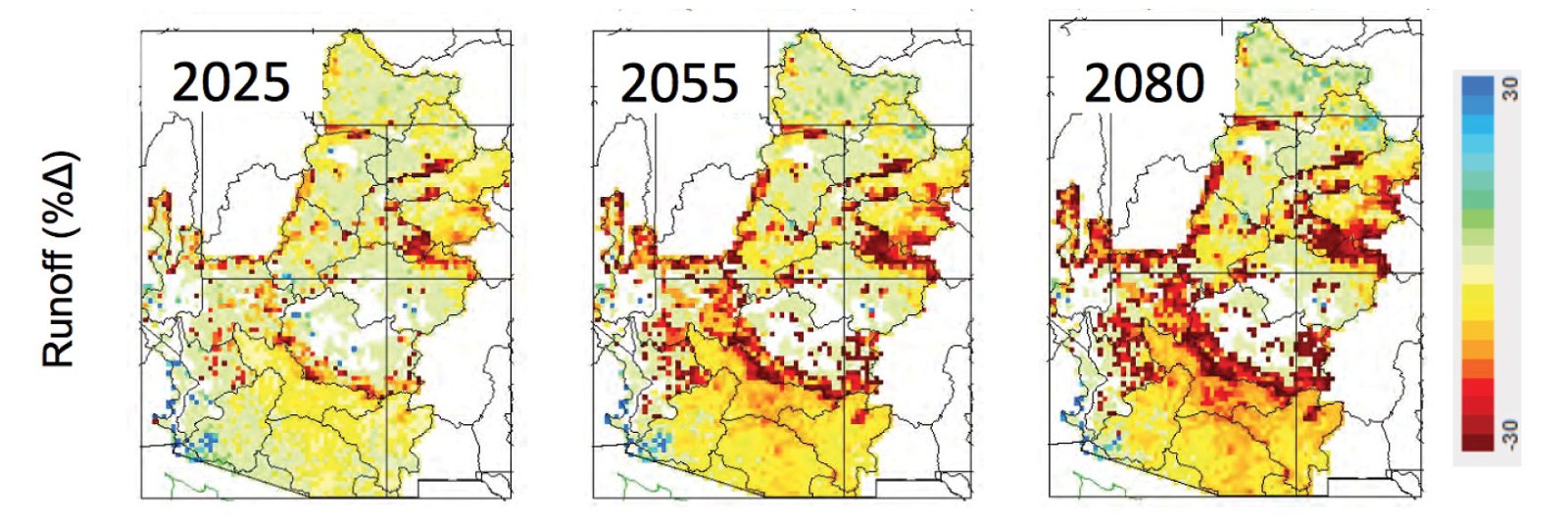
By 2050, our demand for water may outpace supply. This map is a projection based on “business-as-usual” trends in growth, population, and energy demands. It shows the average results from 16 climate models. The darker colors show areas at the highest risk for water shortages if current use patterns continue. In parentheses is the number of counties in each category. Image: “Evaluating Sustainability of Projected Water Demands in 2050 Under Climate Change Scenarios,” Natural Resources Defense Council, 2010

Using History to Prepare for the Future

The Great Flood of 1862 was a massive storm event that impacted California, Nevada, Oregon, Idaho, Utah, and Arizona. 45 straight days of rain led to widespread flooding that ultimately bankrupted the state of California. So many cattle drowned that the state economy shifted from ranching to farming, a trend that persists to this day. The probability of a storm event of this magnitude occurring is about 1 in every 500 to 1,000 years.

The US Geological Survey used the 1862 flood data to create a highly detailed simulation model, called the ArkStorm, to see what would happen if a storm of the same magnitude hit the region again. They showed that, in California alone, the ArkStorm would cause roughly $725 billion dollars worth of damage. That’s nearly 3 times the loss a severe earthquake would cause, an event with a similar probability of occurring.

Understanding devastating events like these is not only critical for planning emergency response. It can also be helpful in water supply forecasting, since major storm events can end a prolonged drought.

1862 Flood

Illustrations of the 1862 flood destruction in Sacramento, CA (left) and Nevada (right)

ArkStorm Simulation

The ArkStorm simulation model showing predicted flood impact in Northern California from a storm event similar to the one experienced in 1862. Image: USGS

When History Doesn’t Reflect the Future

Basin States

The Colorado River Drainage Basin

1922 Basin Allocations

1922 chart used to estimate irrigation and other water requirements for the seven basin states and Mexico for the Colorado River Compact. Notice that Nevada has the lowest allocation. At the time Nevada was only sparsely populated.

The Colorado River and its tributaries provide water to about 40 million people across 7 US and 2 Mexican states. Besides quenching the thirst of millions of people, Colorado River water irrigates about 4 million acres of farmland, and it provides more than 12 billion kilowatt-hours of hydroelectricity each year.

The Colorado River is managed under a hodge-podge of compacts, laws, decrees, and guidelines, now collectively known as the "Law of the River." One of the most significant of these documents is the Colorado River Compact of 1922. This document divided the river basin into two regions—the Upper and Lower Basins—and split the river water between them. Each basin was allowed to take 7.5 million acre-feet per year.

The compact was based on measurements collected between 1905 and 1922. During this period, the river carried an average of 16.1 acre-feet of water per year—more than enough to supply the 15 million acre-feet that the compact allotted.

Unfortunately, the Colorado River Compact was based on poor modeling. What the compact drafters didn’t realize was that the period from 1905 to 1922 was unusually wet. In fact, the river had a higher flow volume during this period than any other in the 20th century. Additionally, measurements of tree rings, which are indicators of past rainfall, show that our recent "drought" patterns are closer to the historical norm. Frequently, the river carries less than the 15 million acre-feet laid out in the compact.

This theoretical deficit hasn’t yet been a problem, because the Upper Basin states—Utah, Wyoming, Colorado, and New Mexico—have not been using their full allocation. California has long benefited from the leftovers. In 1997, for example, California was able to use about 5.2 acre-feet, even though its allocation was just 4.4 million acre-feet.

But these surpluses are drying up. Greater climate variability has made the river’s flow less predictable. Development and population growth have continued. In the face of these increasing pressures, sophisticated predictive modeling is critical for managing the Colorado River into the future.

Predicted Runoff

Predicted Change in Annual Runoff in the Colorado River Basin using the Variable Infiltration Capacity (VIC) model. Image: Colorado River Basin Water Supply and Demand Study–Water Supply Assessment , U. S. Department of the Interior Bureau of Reclamation, February 2012

Water Planning for Increasing Climate Variability

Learn how the Bureau of Reclamation accounts for climate uncertainty when predicting water availability.

Lake Oroville

Lake Oroville, the second-largest reservoir in California, in 2011 (top) and in 2014 (bottom) during a major drought. Image: California Department of Water Resources

For years water resources management has operated under the assumption of “stationarity”—the idea that certain natural phenomena (like temperature and precipitation) will change only within a limited range of possibilities. In other words, variability has limits.

Stationarity further assumes that the probability of any event (like a drought of a certain magnitude) does not change over time. And that those probabilities can be reasonably estimated from prior observations.

Under the assumptions of stationarity, predictive modeling becomes straight-forward. You simply predict that what will happen in the future is what happened in the past. However, changing conditions are challenging these assumptions, and the future of water is becoming increasingly uncertain.

Contributing to uncertainty are things like land use changes, groundwater depletion, and socio-economic fluctuations. One of the biggest sources of uncertainty is climate variability. As the Intergovernmental Panel on Climate Change (IPCC) puts it, “Climate change challenges the traditional assumption that past hydrological experience provides a good guide to future conditions.”

Climate variability widens the range of possible extremes. It amplifies the limitations of observational records and invalidates historical assumptions. In the face of climate variability, predictive modeling for water becomes much more difficult.

To account for uncertainty, water managers have developed new approaches to plan for a growing range of potential future conditions. Improved predictive modeling helps managers identify areas of vulnerability, prepare communities for more possibilities, and develop plans for coping with whatever the future climate will do.

Snowmelt in the West

In the Intermountain West, snow buildup in mountain watersheds serves as a massive natural reservoir. Snowmelt from the Rocky mountains of Wyoming and Colorado supplies the bulk of the Colorado River's water. In Salt Lake City’s watershed (a separate drainage), over 80% of the surface water supply comes from snowmelt.

Snowmelt follows a yearly cycle. In the Colorado River Basin, melting usually begins in April, peaks during May and June, and tapers off around late July or early August.

In recent years, however, temperatures across the western US have increased. A greater proportion of winter precipitation has been falling as rain, and snow has been melting earlier in the season. Models predict that if these temperature trends continue, early runoff could bring too much water to reservoirs early in the year and leave too little for later. Higher temperatures would also limit snowfall to higher elevations, decreasing the mountains' holding capacity.

Rapid snowmelt can cause erosion and flooding. Snowmelt predictive models show how the timing and extent of snowmelt might change in different terrain and climate conditions. This information can help water managers make better decisions. It can also help in forecasting floods

Snowmelt

July snowmelt in Boulder, Colorado Image: Jessee Varner

Snow Model

Snowmelt is a vital water source in the intermountain west. Water managers use snowmelt predictive model simulations like this one to predict snowmelt runoff. Image: The Gridded Surface Subsurface Hydrologic Analysis (GSSHA) model developed by U.S. Army Corps of Engineers Engineer Research and Development Center (ERDC) and Aquaveo, LLC

References

References

Olsen, J. Rolf, Julie Kiang and Reagan Waskom, (editors). 2010. Workshop on Nonstationarity, Hydrologic Frequency Analysis, and Water Management. Colorado Water Institute Information Series No. 109. http://www.cwi.colostate.edu

U.S. Department of the Interior, Bureau of Reclamation. (2012). Colorado River Basin: Water Supply and Demand Study Technical Report C – Water Demand Assessment. http://www.usbr.gov/lc/region/programs/crbstudy/finalreport/techrptC.html

Donkor, E. A., Mazzuchi, T. A., Soyer, R., & Alan Roberson, J. (2012). Urban water demand forecasting: review of methods and models. Journal of Water Resources Planning and Management, 140(2), 146-159.

Milly, P. C. D., Julio, B., Malin, F., Robert, M., Zbigniew, W., Dennis, P., & Ronald, J. S. (2007). Stationarity is dead. Ground Water News & Views, 4(1), 6-8.

Roy, S. B., Chen, L., Girvetz, E., Maurer, E. P., Mills, W. B., & Grieb, T. M. (2010). Evaluating sustainability of projected water demands under future climate change scenarios. New York: Natural Resources Defense Council.


APA format:

Genetic Science Learning Center. (2015, March 15) What the Future Holds. Retrieved April 15, 2024, from https://learn.genetics.utah.edu/content/earth/future

CSE format:

What the Future Holds [Internet]. Salt Lake City (UT): Genetic Science Learning Center; 2015 [cited 2024 Apr 15] Available from https://learn.genetics.utah.edu/content/earth/future

Chicago format:

Genetic Science Learning Center. "What the Future Holds." Learn.Genetics. March 15, 2015. Accessed April 15, 2024. https://learn.genetics.utah.edu/content/earth/future.